Um novo pacote do R para análise descritiva
O Pacote dlookr
Na documentação do pacote podemos ver o objetivo desse pacote: Diagnosticar, explorar e transformar dados.
Recursos: 1. Diagnosticar a qualidade dos dados. 2. Explorar e compreender de dados. 3. Criar novas variáveis e/ou executar transformações de variáveis. 4. Gerar relatórios automaticamente.
Para mostrar o funcionamento do pacote, vamos usar a base de dados CARROS
load(url("https://github.com/DATAUNIRIO/Base_de_dados/raw/master/CARROS.RData"))
ls()
## [1] "CARROS"CARROS$Tipodecombustivel<-ifelse(CARROS$Tipodecombustivel==0,"Gas","Alc")
CARROS$TipodeMarcha<-ifelse(CARROS$TipodeMarcha==0,"Auto","Manual")
CARROS$Tipodecombustivel<-as.factor(CARROS$Tipodecombustivel)
CARROS$TipodeMarcha<-as.factor(CARROS$TipodeMarcha)Vamos ver algumas funções do pacote. Um consideração importante é que ele pode ser integrado ao tidyverse.
# https://github.com/choonghyunryu/dlookr
# install.packages("dlookr")

library("dlookr")

diagnose(CARROS)
## # A tibble: 11 x 6
## variables types missing_count missing_percent unique_count unique_rate
## <chr> <chr> <int> <dbl> <int> <dbl>
## 1 Kmporlitro nume~ 0 0 25 0.781
## 2 Cilindros nume~ 0 0 3 0.0938
## 3 Preco nume~ 0 0 27 0.844
## 4 HP nume~ 0 0 22 0.688
## 5 Amperagem_circ_~ nume~ 0 0 22 0.688
## 6 Peso nume~ 0 0 29 0.906
## 7 RPM nume~ 0 0 30 0.938
## 8 Tipodecombustiv~ fact~ 0 0 2 0.0625
## 9 TipodeMarcha fact~ 0 0 2 0.0625
## 10 NumdeMarchas nume~ 0 0 3 0.0938
## 11 NumdeValvulas nume~ 0 0 6 0.188# Select columns by name
diagnose(CARROS, Kmporlitro, HP, TipodeMarcha)## # A tibble: 3 x 6
## variables types missing_count missing_percent unique_count unique_rate
## <chr> <chr> <int> <dbl> <int> <dbl>
## 1 Kmporlitro numeric 0 0 25 0.781
## 2 HP numeric 0 0 22 0.688
## 3 TipodeMarcha factor 0 0 2 0.0625# Diagnosis of numeric variables with diagnose_numeric()
diagnose_numeric(CARROS)## # A tibble: 9 x 10
## variables min Q1 mean median Q3 max zero minus outlier
## <chr> <dbl> <dbl> <dbl> <dbl> <dbl> <dbl> <int> <int> <int>
## 1 Kmporlitro 10.4 15.4 20.1 19.2 22.8 33.9 0 0 0
## 2 Cilindros 4 4 6.19 6 8 8 0 0 0
## 3 Preco 71.1 121. 231. 196. 326 472 0 0 0
## 4 HP 52 96.5 147. 123 180 335 0 0 1
## 5 Amperagem_circ_e~ 2.76 3.08 3.60 3.70 3.92 4.93 0 0 0
## 6 Peso 1.51 2.58 3.22 3.32 3.61 5.42 0 0 2
## 7 RPM 14.5 16.9 17.8 17.7 18.9 22.9 0 0 1
## 8 NumdeMarchas 3 3 3.69 4 4 5 0 0 0
## 9 NumdeValvulas 1 2 2.81 2 4 8 0 0 1Um exemplo de integração com o dplyr.
library(dplyr)
CARROS %>%
  select(Kmporlitro, HP) %>%
  filter(Kmporlitro > 20 | HP > 100) %>%
  diagnose_numeric()
## # A tibble: 2 x 10
## variables min Q1 mean median Q3 max zero minus outlier
## <chr> <dbl> <dbl> <dbl> <dbl> <dbl> <dbl> <int> <int> <int>
## 1 Kmporlitro 10.4 15.4 20.1 19.2 22.8 33.9 0 0 0
## 2 HP 52 96.5 147. 123 180 335 0 0 1# Diagnosis of categorical variables with diagnose_category()
diagnose_category(CARROS)## variables levels N freq ratio rank
## 1 Tipodecombustivel Gas 32 18 56.250 1
## 2 Tipodecombustivel Alc 32 14 43.750 2
## 3 TipodeMarcha Auto 32 19 59.375 1
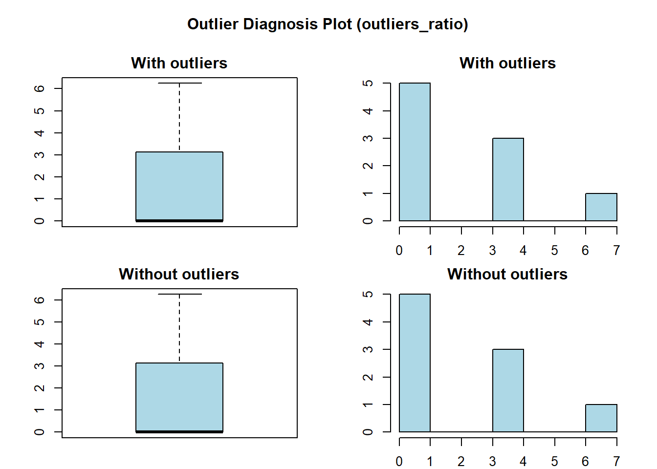
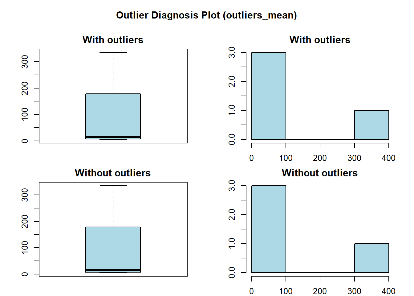
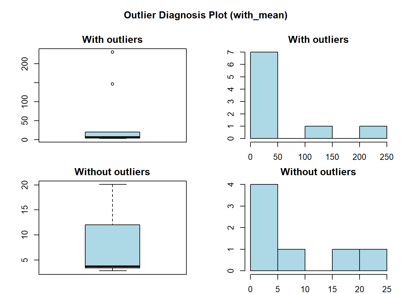
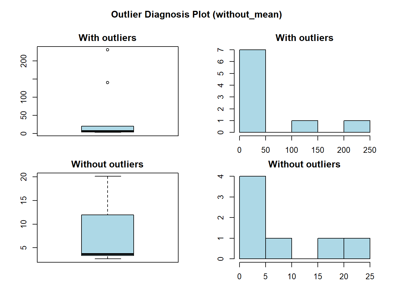
## 4 TipodeMarcha Manual 32 13 40.625 2Os outliers
# Diagnosing outliers with diagnose_outlier()
diagnose_outlier(CARROS)
## variables outliers_cnt outliers_ratio outliers_mean with_mean
## 1 Kmporlitro 0 0.000 NaN 20.090625
## 2 Cilindros 0 0.000 NaN 6.187500
## 3 Preco 0 0.000 NaN 230.721875
## 4 HP 1 3.125 335.0000 146.687500
## 5 Amperagem_circ_eletrico 0 0.000 NaN 3.596563
## 6 Peso 2 6.250 5.3845 3.217250
## 7 RPM 1 3.125 22.9000 17.848750
## 8 NumdeMarchas 0 0.000 NaN 3.687500
## 9 NumdeValvulas 1 3.125 8.0000 2.812500
## without_mean
## 1 20.090625
## 2 6.187500
## 3 230.721875
## 4 140.612903
## 5 3.596563
## 6 3.072767
## 7 17.685806
## 8 3.687500
## 9 2.645161# Visualization of outliers using plot_outlier()
plot_outlier(diagnose_outlier(CARROS))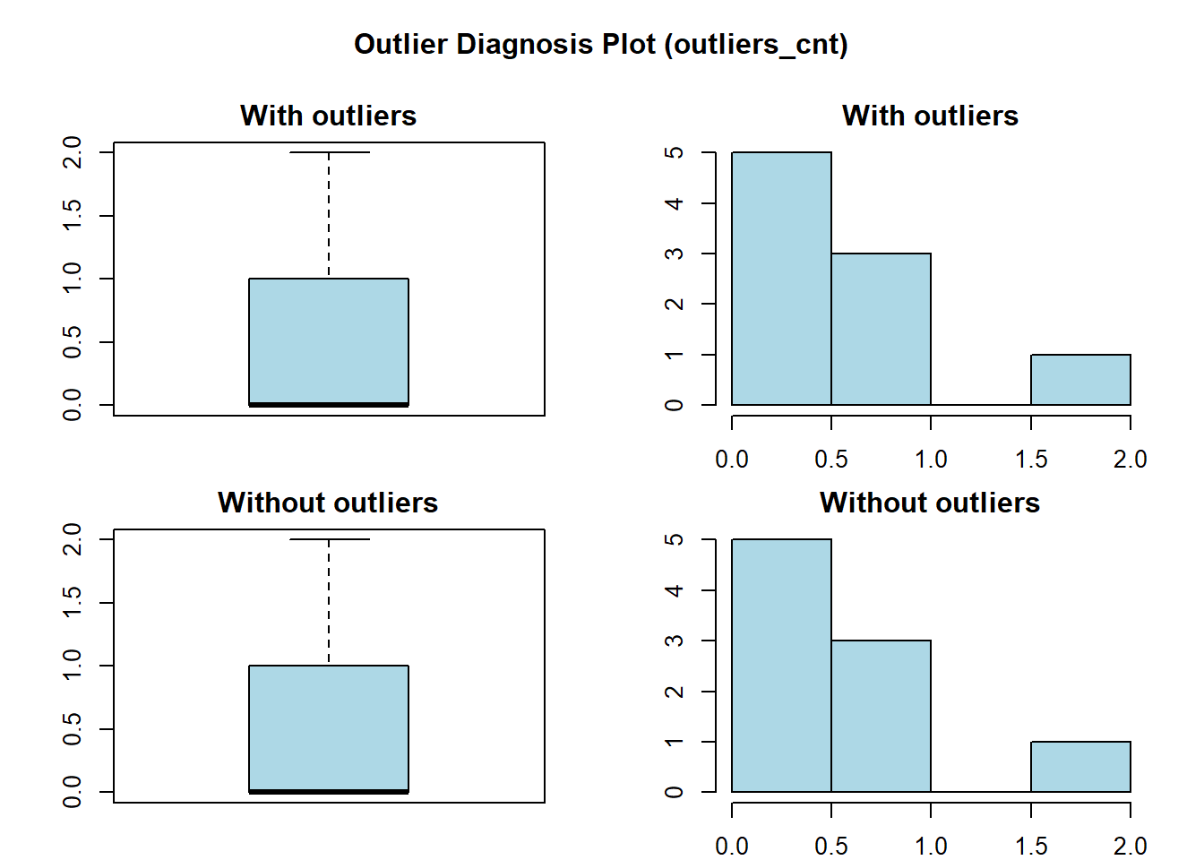
Análise Descritiva
describe(CARROS)## # A tibble: 9 x 26
## variable n na mean sd se_mean IQR skewness kurtosis p00
## <chr> <int> <int> <dbl> <dbl> <dbl> <dbl> <dbl> <dbl> <dbl>
## 1 Kmporli~ 32 0 20.1 6.03 1.07 7.38 0.672 -0.0220 10.4
## 2 Cilindr~ 32 0 6.19 1.79 0.316 4 -0.192 -1.76 4
## 3 Preco 32 0 231. 124. 21.9 205. 0.420 -1.07 71.1
## 4 HP 32 0 147. 68.6 12.1 83.5 0.799 0.275 52
## 5 Amperag~ 32 0 3.60 0.535 0.0945 0.840 0.293 -0.450 2.76
## 6 Peso 32 0 3.22 0.978 0.173 1.03 0.466 0.417 1.51
## 7 RPM 32 0 17.8 1.79 0.316 2.01 0.406 0.865 14.5
## 8 NumdeMa~ 32 0 3.69 0.738 0.130 1 0.582 -0.895 3
## 9 NumdeVa~ 32 0 2.81 1.62 0.286 2 1.16 2.02 1
## # ... with 16 more variables: p01 <dbl>, p05 <dbl>, p10 <dbl>, p20 <dbl>,
## # p25 <dbl>, p30 <dbl>, p40 <dbl>, p50 <dbl>, p60 <dbl>, p70 <dbl>,
## # p75 <dbl>, p80 <dbl>, p90 <dbl>, p95 <dbl>, p99 <dbl>, p100 <dbl>CARROS %>%
describe() %>%
select(variable, mean, p25, p50, p75) %>%
filter(!is.na(mean)) %>%
arrange(desc(abs(mean)))## # A tibble: 9 x 5
## variable mean p25 p50 p75
## <chr> <dbl> <dbl> <dbl> <dbl>
## 1 Preco 231. 121. 196. 326
## 2 HP 147. 96.5 123 180
## 3 Kmporlitro 20.1 15.4 19.2 22.8
## 4 RPM 17.8 16.9 17.7 18.9
## 5 Cilindros 6.19 4 6 8
## 6 NumdeMarchas 3.69 3 4 4
## 7 Amperagem_circ_eletrico 3.60 3.08 3.70 3.92
## 8 Peso 3.22 2.58 3.32 3.61
## 9 NumdeValvulas 2.81 2 2 4CARROS %>%
group_by(Tipodecombustivel) %>%
describe(Kmporlitro, HP) ## # A tibble: 4 x 27
## variable Tipodecombustiv~ n na mean sd se_mean IQR skewness
## <chr> <fct> <dbl> <dbl> <dbl> <dbl> <dbl> <dbl> <dbl>
## 1 Kmporli~ Alc 14 0 24.6 5.38 1.44 8.22 0.510
## 2 Kmporli~ Gas 18 0 16.6 3.86 0.910 4.3 0.578
## 3 HP Alc 14 0 91.4 24.4 6.53 43.8 -0.301
## 4 HP Gas 18 0 190. 60.3 14.2 70 0.539
## # ... with 18 more variables: kurtosis <dbl>, p00 <dbl>, p01 <dbl>, p05 <dbl>,
## # p10 <dbl>, p20 <dbl>, p25 <dbl>, p30 <dbl>, p40 <dbl>, p50 <dbl>,
## # p60 <dbl>, p70 <dbl>, p75 <dbl>, p80 <dbl>, p90 <dbl>, p95 <dbl>,
## # p99 <dbl>, p100 <dbl>CARROS %>%
group_by(Tipodecombustivel) %>%
diagnose_category(TipodeMarcha)## # A tibble: 4 x 7
## # Groups: Tipodecombustivel [2]
## Tipodecombustivel variables levels N freq ratio rank
## <fct> <chr> <fct> <int> <int> <dbl> <int>
## 1 Gas TipodeMarcha Auto 18 12 66.7 1
## 2 Alc TipodeMarcha Auto 14 7 50 1
## 3 Alc TipodeMarcha Manual 14 7 50 2
## 4 Gas TipodeMarcha Manual 18 6 33.3 2CARROS %>%
group_by(Tipodecombustivel) %>%
diagnose_category()## # A tibble: 6 x 8
## # Groups: variable [3]
## variable variables levels N freq ratio rank Tipodecombustivel
## <fct> <chr> <fct> <int> <int> <dbl> <int> <fct>
## 1 Gas Tipodecombustivel Gas 18 18 100 1 <NA>
## 2 Alc Tipodecombustivel Alc 14 14 100 1 <NA>
## 3 <NA> TipodeMarcha Auto 18 12 66.7 1 Gas
## 4 <NA> TipodeMarcha Auto 14 7 50 1 Alc
## 5 <NA> TipodeMarcha Manual 14 7 50 2 Alc
## 6 <NA> TipodeMarcha Manual 18 6 33.3 2 GasNormalidade
normality(CARROS)## # A tibble: 9 x 4
## vars statistic p_value sample
## <chr> <dbl> <dbl> <dbl>
## 1 Kmporlitro 0.948 0.123 32
## 2 Cilindros 0.753 0.00000606 32
## 3 Preco 0.920 0.0208 32
## 4 HP 0.933 0.0488 32
## 5 Amperagem_circ_eletrico 0.946 0.110 32
## 6 Peso 0.943 0.0927 32
## 7 RPM 0.973 0.594 32
## 8 NumdeMarchas 0.773 0.0000131 32
## 9 NumdeValvulas 0.851 0.000438 32CARROS %>%
normality() %>%
filter(p_value <= 0.05) %>%
arrange(abs(p_value))## # A tibble: 5 x 4
## vars statistic p_value sample
## <chr> <dbl> <dbl> <dbl>
## 1 Cilindros 0.753 0.00000606 32
## 2 NumdeMarchas 0.773 0.0000131 32
## 3 NumdeValvulas 0.851 0.000438 32
## 4 Preco 0.920 0.0208 32
## 5 HP 0.933 0.0488 32CARROS %>%
group_by(Tipodecombustivel) %>%
normality(Kmporlitro) %>%
arrange(desc(p_value))## # A tibble: 2 x 5
## variable Tipodecombustivel statistic p_value sample
## <chr> <fct> <dbl> <dbl> <dbl>
## 1 Kmporlitro Gas 0.952 0.449 18
## 2 Kmporlitro Alc 0.912 0.167 14CARROS %>%
mutate(log_hp = log(HP)) %>%
group_by(Tipodecombustivel) %>%
normality(log_hp) %>%
filter(p_value > 0.05)## # A tibble: 2 x 5
## variable Tipodecombustivel statistic p_value sample
## <chr> <fct> <dbl> <dbl> <dbl>
## 1 log_hp Alc 0.880 0.0589 14
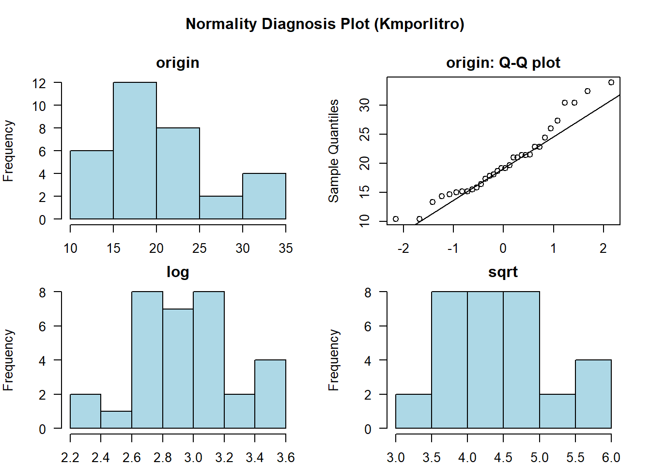
## 2 log_hp Gas 0.959 0.591 18# Select columns by name
plot_normality(CARROS, HP, Kmporlitro)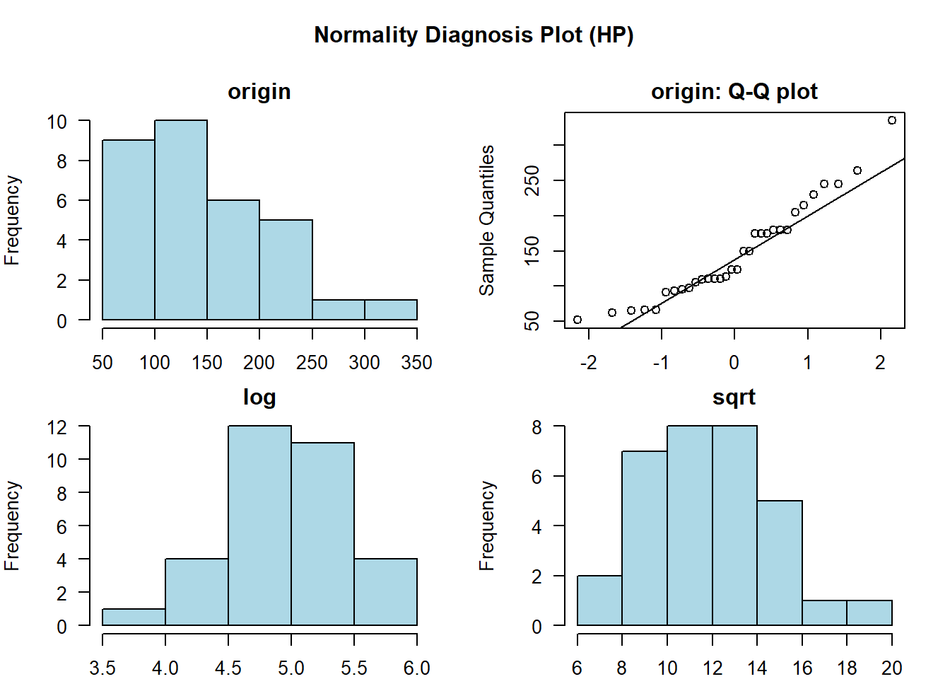
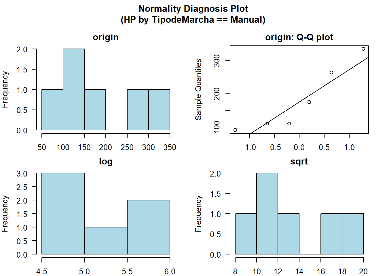
CARROS %>%
  filter(Tipodecombustivel == "Gas") %>%
  group_by(TipodeMarcha) %>%
  plot_normality(HP)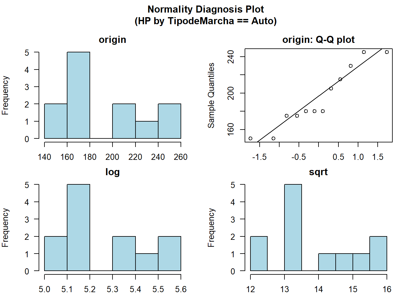
Correlação
correlate(CARROS)## # A tibble: 72 x 3
## var1 var2 coef_corr
## <fct> <fct> <dbl>
## 1 Cilindros Kmporlitro -0.852
## 2 Preco Kmporlitro -0.848
## 3 HP Kmporlitro -0.776
## 4 Amperagem_circ_eletrico Kmporlitro 0.681
## 5 Peso Kmporlitro -0.868
## 6 RPM Kmporlitro 0.419
## 7 NumdeMarchas Kmporlitro 0.480
## 8 NumdeValvulas Kmporlitro -0.551
## 9 Kmporlitro Cilindros -0.852
## 10 Preco Cilindros 0.902
## # ... with 62 more rowsplot_correlate(CARROS)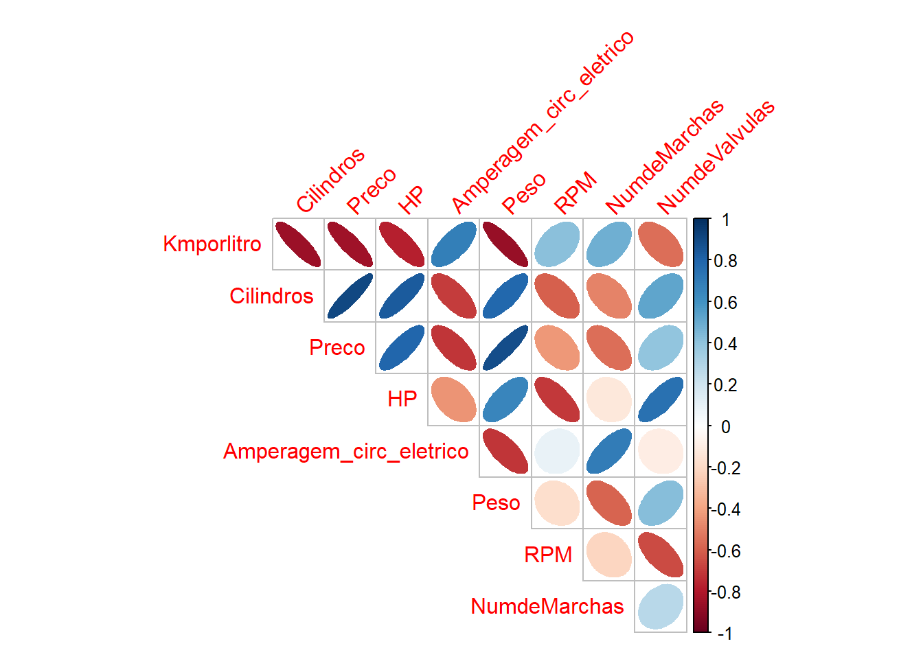
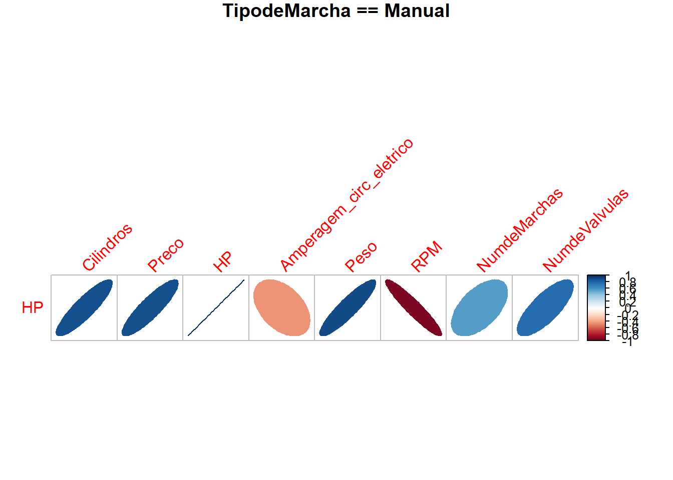
CARROS %>%
  filter(Tipodecombustivel == "Gas") %>%
  group_by(TipodeMarcha) %>%
  plot_correlate(HP)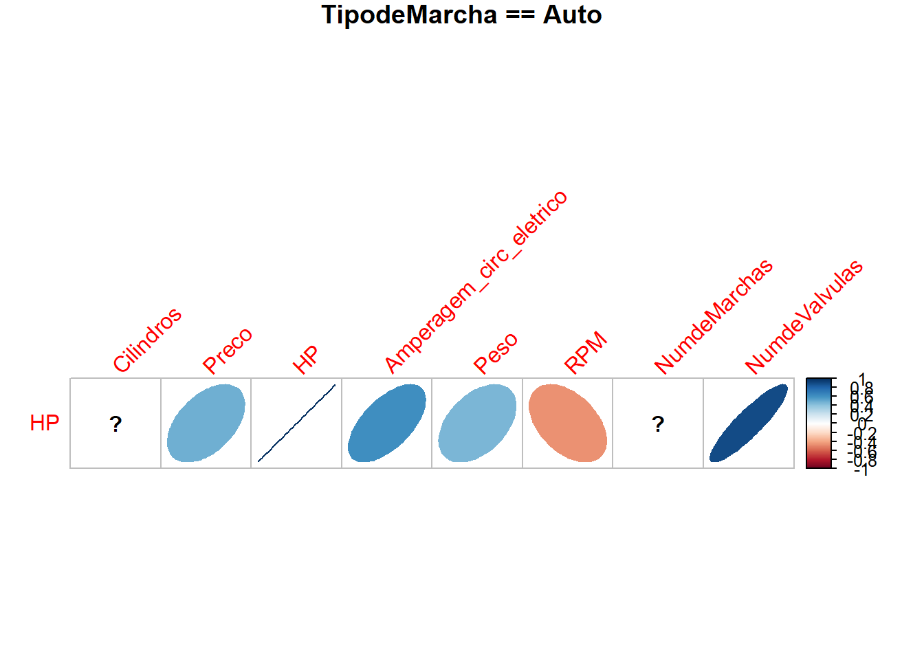
Análise Exploratória de dados
# EDA based on target variable
# Definition of target variable
categ <- target_by(CARROS, Tipodecombustivel)

# If the variable of interest is a numerical variable
cat_num <- relate(categ, HP)
cat_num
## # A tibble: 3 x 27
## variable Tipodecombustiv~ n na mean sd se_mean IQR skewness
## <chr> <fct> <dbl> <dbl> <dbl> <dbl> <dbl> <dbl> <dbl>
## 1 HP Alc 14 0 91.4 24.4 6.53 43.8 -0.301
## 2 HP Gas 18 0 190. 60.3 14.2 70 0.539
## 3 HP total 32 0 147. 68.6 12.1 83.5 0.799
## # ... with 18 more variables: kurtosis <dbl>, p00 <dbl>, p01 <dbl>, p05 <dbl>,
## # p10 <dbl>, p20 <dbl>, p25 <dbl>, p30 <dbl>, p40 <dbl>, p50 <dbl>,
## # p60 <dbl>, p70 <dbl>, p75 <dbl>, p80 <dbl>, p90 <dbl>, p95 <dbl>,
## # p99 <dbl>, p100 <dbl>summary(cat_num)## variable Tipodecombustivel n na
## Length:3 Alc :1 Min. :14.00 Min. :0
## Class :character Gas :1 1st Qu.:16.00 1st Qu.:0
## Mode :character total:1 Median :18.00 Median :0
## Mean :21.33 Mean :0
## 3rd Qu.:25.00 3rd Qu.:0
## Max. :32.00 Max. :0
## mean sd se_mean IQR
## Min. : 91.36 Min. :24.42 Min. : 6.528 Min. :43.75
## 1st Qu.:119.02 1st Qu.:42.35 1st Qu.: 9.324 1st Qu.:56.88
## Median :146.69 Median :60.28 Median :12.120 Median :70.00
## Mean :142.59 Mean :51.09 Mean :10.952 Mean :65.75
## 3rd Qu.:168.20 3rd Qu.:64.42 3rd Qu.:13.164 3rd Qu.:76.75
## Max. :189.72 Max. :68.56 Max. :14.208 Max. :83.50
## skewness kurtosis p00 p01
## Min. :-0.3014 Min. :-1.4580 Min. :52.0 Min. :53.30
## 1st Qu.: 0.1190 1st Qu.:-0.5914 1st Qu.:52.0 1st Qu.:54.20
## Median : 0.5394 Median : 0.2752 Median :52.0 Median :55.10
## Mean : 0.3458 Mean :-0.1626 Mean :65.0 Mean :67.54
## 3rd Qu.: 0.6694 3rd Qu.: 0.4851 3rd Qu.:71.5 3rd Qu.:74.67
## Max. : 0.7994 Max. : 0.6950 Max. :91.0 Max. :94.23
## p05 p10 p20 p25
## Min. : 58.50 Min. : 62.90 Min. : 65.6 Min. : 66.00
## 1st Qu.: 61.08 1st Qu.: 64.45 1st Qu.: 79.5 1st Qu.: 81.25
## Median : 63.65 Median : 66.00 Median : 93.4 Median : 96.50
## Mean : 76.43 Mean : 79.63 Mean :103.0 Mean :106.25
## 3rd Qu.: 85.40 3rd Qu.: 88.00 3rd Qu.:121.7 3rd Qu.:126.38
## Max. :107.15 Max. :110.00 Max. :150.0 Max. :156.25
## p30 p40 p50 p60
## Min. : 66.0 Min. : 93.4 Min. : 96.0 Min. :103.4
## 1st Qu.: 86.1 1st Qu.:101.7 1st Qu.:109.5 1st Qu.:134.2
## Median :106.2 Median :110.0 Median :123.0 Median :165.0
## Mean :115.7 Mean :126.1 Mean :133.0 Mean :151.1
## 3rd Qu.:140.6 3rd Qu.:142.5 3rd Qu.:151.5 3rd Qu.:175.0
## Max. :175.0 Max. :175.0 Max. :180.0 Max. :185.0
## p70 p75 p80 p90
## Min. :109.1 Min. :109.8 Min. :111.2 Min. :120.0
## 1st Qu.:143.8 1st Qu.:144.9 1st Qu.:155.6 1st Qu.:181.8
## Median :178.5 Median :180.0 Median :200.0 Median :243.5
## Mean :167.2 Mean :172.0 Mean :183.4 Mean :204.7
## 3rd Qu.:196.2 3rd Qu.:203.1 3rd Qu.:219.5 3rd Qu.:247.1
## Max. :214.0 Max. :226.2 Max. :239.0 Max. :250.7
## p95 p99 p100
## Min. :123.0 Min. :123.0 Min. :123.0
## 1st Qu.:188.3 1st Qu.:218.0 1st Qu.:229.0
## Median :253.6 Median :313.0 Median :335.0
## Mean :217.1 Mean :253.0 Mean :264.3
## 3rd Qu.:264.1 3rd Qu.:318.0 3rd Qu.:335.0
## Max. :274.6 Max. :322.9 Max. :335.0plot(cat_num)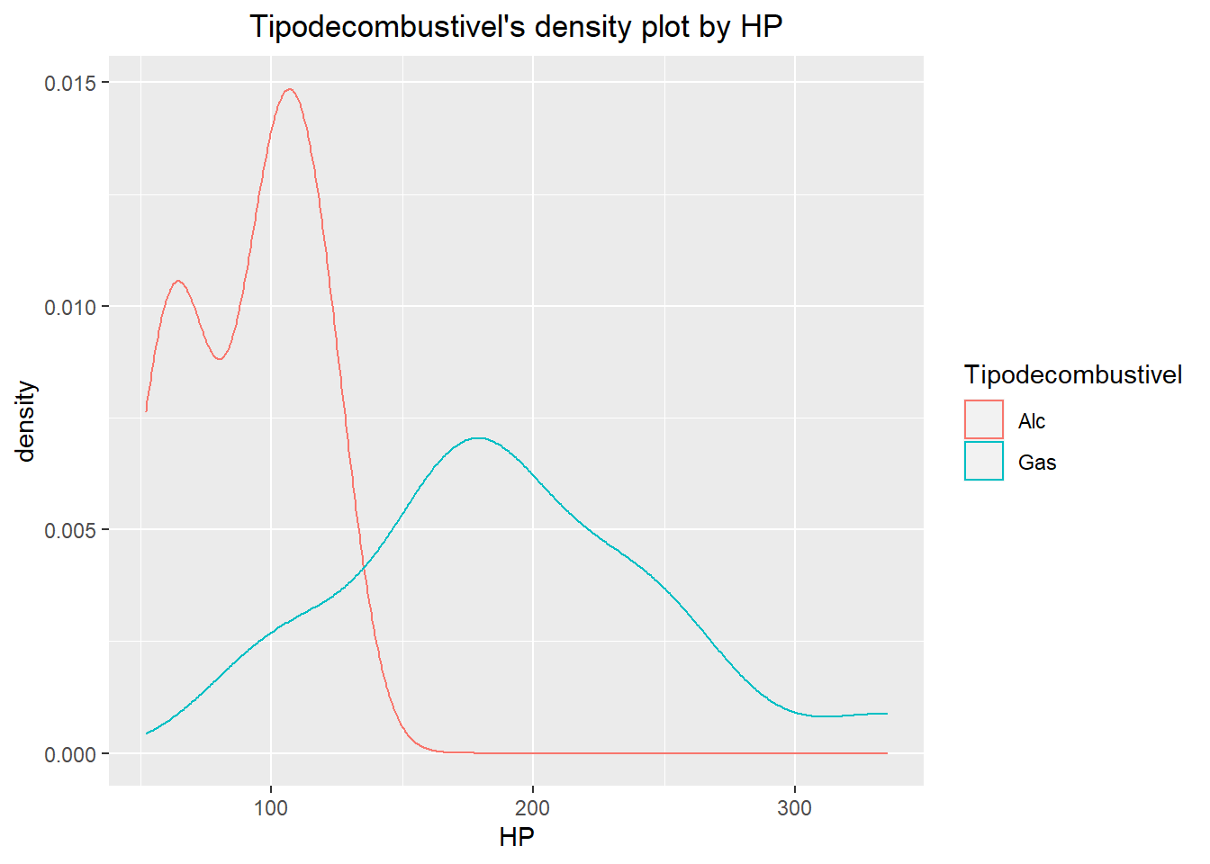
# If the variable of interest is a categorical variable
cat_cat <- relate(categ, TipodeMarcha)
cat_cat
## TipodeMarcha
## Tipodecombustivel Auto Manual
## Alc 7 7
## Gas 12 6summary(cat_cat)## Call: xtabs(formula = formula_str, data = data, addNA = TRUE)
## Number of cases in table: 32
## Number of factors: 2
## Test for independence of all factors:
## Chisq = 0.9069, df = 1, p-value = 0.3409plot(cat_cat)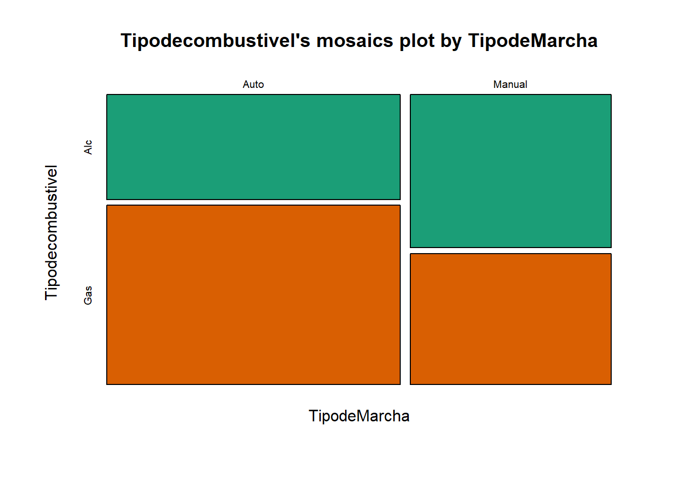
# EDA when target variable is numerical variable
# If the variable of interest is a numerical variable
num <- target_by(CARROS, HP)
# If the variable of interest is a numerical variable
num_num <- relate(num, Kmporlitro)
num_num
##
## Call:
## lm(formula = formula_str, data = data)
##
## Coefficients:
## (Intercept) Kmporlitro
## 324.08 -8.83summary(num_num)##
## Call:
## lm(formula = formula_str, data = data)
##
## Residuals:
## Min 1Q Median 3Q Max
## -59.26 -28.93 -13.45 25.65 143.36
##
## Coefficients:
## Estimate Std. Error t value Pr(>|t|)
## (Intercept) 324.08 27.43 11.813 8.25e-13 ***
## Kmporlitro -8.83 1.31 -6.742 1.79e-07 ***
## ---
## Signif. codes: 0 '***' 0.001 '**' 0.01 '*' 0.05 '.' 0.1 ' ' 1
##
## Residual standard error: 43.95 on 30 degrees of freedom
## Multiple R-squared: 0.6024, Adjusted R-squared: 0.5892
## F-statistic: 45.46 on 1 and 30 DF, p-value: 1.788e-07plot(num_num)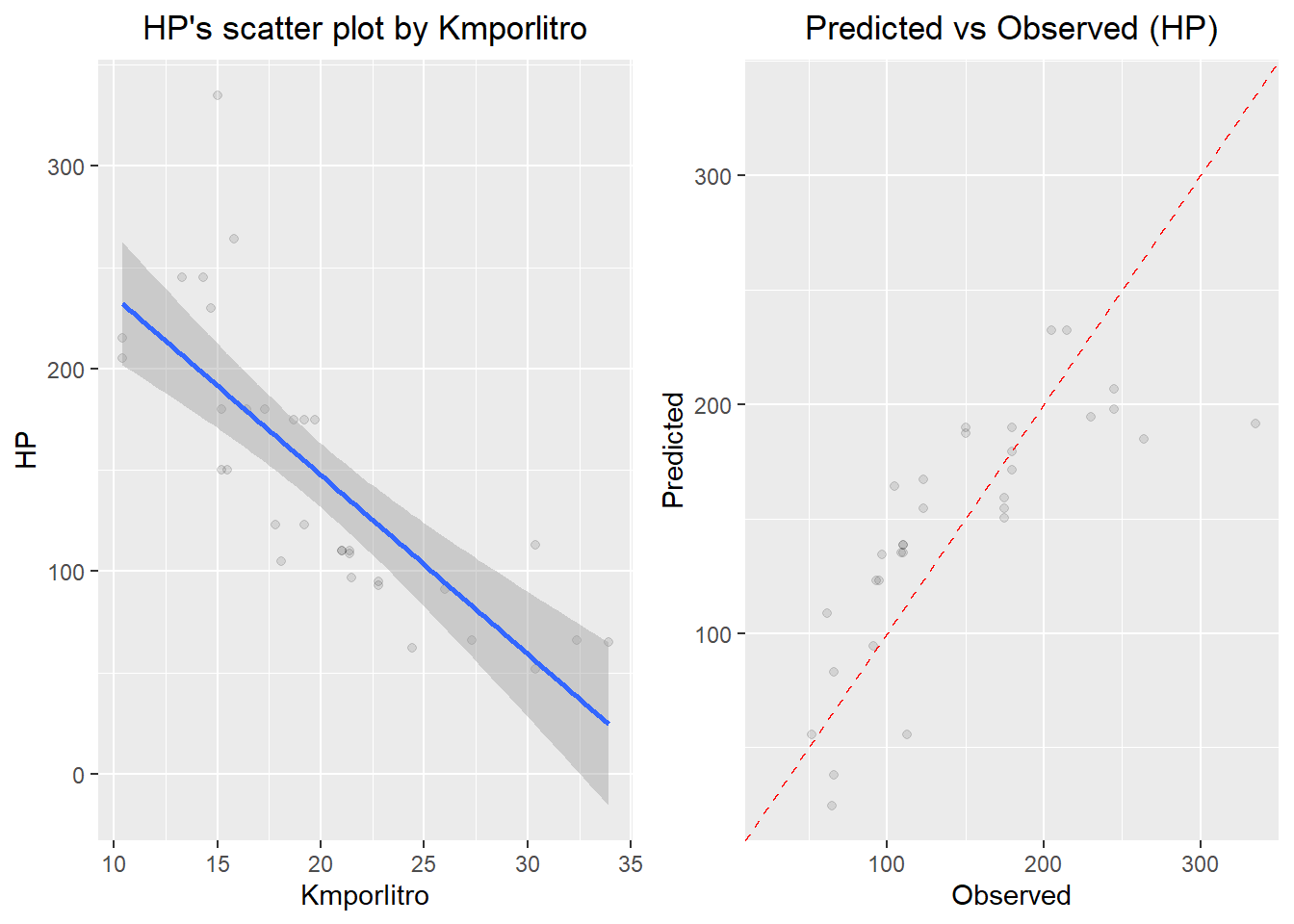
# If the variable of interest is a categorical variable
num_cat <- relate(num, Tipodecombustivel)
num_cat
## Analysis of Variance Table
##
## Response: HP
## Df Sum Sq Mean Sq F value Pr(>F)
## Tipodecombustivel 1 76196 76196 32.876 2.941e-06 ***
## Residuals 30 69531 2318
## ---
## Signif. codes: 0 '***' 0.001 '**' 0.01 '*' 0.05 '.' 0.1 ' ' 1plot(num_cat)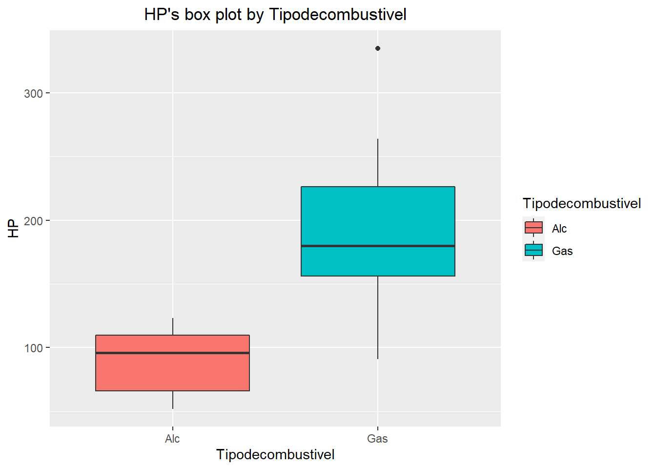
Transformação de dados
a função transform() realiza a transformação dos dados. Apenas variáveis numéricas podem ser utilizadas. Existem dois métodos de transformação:
- “Zscore”: transformação de z-score. (x - mu) / sigma
- “Minmax”: transformação minmax. (x - min) / (max - min)
CARROS %>%
  mutate(kml_minmax = transform(CARROS$Kmporlitro, method = "minmax"),
          hp_minmax = transform(CARROS$HP, method = "minmax")) %>%
  select(kml_minmax, hp_minmax) %>%
  boxplot()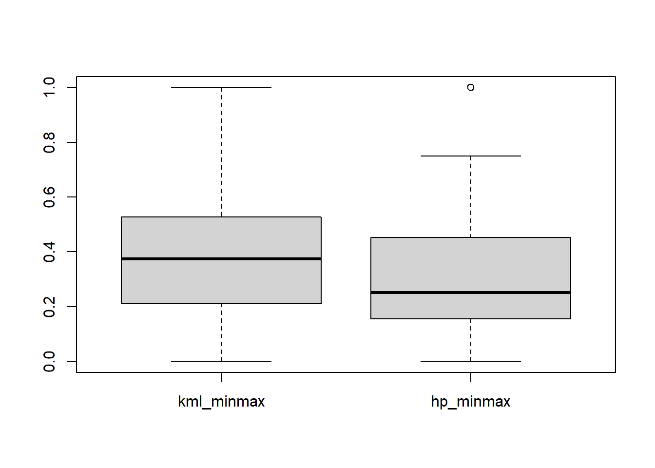
Relatório automáticos
CARROS %>%
  diagnose_report(output_format = "html")

CARROS %>%
  eda_report(target = Kmporlitro)